jeffrey@penn:~/blog$ glow z-transform.md
The Z transform
The Z transform is the discrete-time version of the Laplace transform. It is the tool for sampled signals and digital filters.
Definition
For a discrete-time signal ,
Example: a geometric sequence
For , the geometric series gives
There is a pole at , and the region of convergence is everything outside the circle of radius .
Relation to the Fourier and Laplace transforms
On the unit circle the Z transform becomes the discrete-time Fourier transform (DTFT), the discrete counterpart of the Fourier transform.
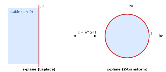
Sampling every seconds and taking the Laplace transform of the samples gives the Z transform with
This maps the axis onto the unit circle and the left half-plane onto the inside of the unit circle. So the stability rule “poles in the left half-plane” becomes “poles inside the unit circle”.
Properties
| Property | Time domain | domain |
|---|---|---|
| Linearity | ||
| Delay | ||
| Difference | ||
| Convolution |
The delay rule turns difference equations into algebra. The filter becomes , so : stable exactly when the pole .
---
title: "The Z transform"
date: 2026-11-01
tags: [signal-processing, math, tutorial, control]
---
The Z transform is the discrete-time version of the [Laplace transform](/blog/laplace-transform/). It is the tool for sampled signals and digital filters.
## Definition
For a discrete-time signal $x[n]$,
$$
X(z) = \mathcal{Z}\{x[n]\} = \sum_{n=-\infty}^{\infty} x[n]\, z^{-n}, \qquad z \in \mathbb{C}.
$$
## Example: a geometric sequence
For $x[n] = a^{n} u[n]$, the geometric series gives
$$
X(z) = \sum_{n=0}^{\infty} \left(a z^{-1}\right)^{n} = \frac{1}{1 - a z^{-1}}, \qquad |z| > |a| .
$$
There is a pole at $z = a$, and the region of convergence is everything outside the circle of radius $|a|$.
## Relation to the Fourier and Laplace transforms
On the unit circle $z = e^{j\Omega}$ the Z transform becomes the discrete-time Fourier transform (DTFT), the discrete counterpart of the [Fourier transform](/blog/fourier-transform/).
Sampling $x(t)$ every $T$ seconds and taking the Laplace transform of the samples gives the Z transform with
$$
z = e^{sT}.
$$
This maps the $j\omega$ axis onto the unit circle and the left half-plane onto the inside of the unit circle. So the stability rule "poles in the left half-plane" becomes "poles inside the unit circle".

## Properties
| Property | Time domain | $z$ domain |
|----------|-------------|------------|
| Linearity | $a x_1[n] + b x_2[n]$ | $a X_1(z) + b X_2(z)$ |
| Delay | $x[n - k]$ | $z^{-k} X(z)$ |
| Difference | $x[n] - x[n-1]$ | $(1 - z^{-1}) X(z)$ |
| Convolution | $(x * h)[n]$ | $X(z) H(z)$ |
The delay rule turns difference equations into algebra. The filter $y[n] = a\, y[n-1] + x[n]$ becomes $Y(z) = a z^{-1} Y(z) + X(z)$, so $H(z) = \frac{1}{1 - a z^{-1}}$: stable exactly when the pole $|a| < 1$.